To make resampling faster, we have implemented two “tweaks” to the process. In the current implementation of the software, you can turn these both on or both off at the same time only. The control is the “Always use full resampling” checkbox in the analysis setup wizard (step 5).
1. Sparse sampling of larger gene set sizes
The background distribution of scores tends to get narrower for larger gene set sizes. Intuitively, if you are only choosing two items from the data, the possibility of getting an extreme value for their average is much higher than if you chose 100 items.
This implies that we can’t just use one background distribution for all gene sets.
In our original implementation of the algorithm, a background distribution was generated for each gene set size. Thus if you analyze sizes from 4 to 100, 97 different resampling runs have to be performed.
Because each run requires computation of a summary statistic for n items, where n is the gene set size, the time this takes increases as the gene set sizes increase. (increasing on the order of n 2 for the correlation scores) .
To reduce this problem, we make use of the fact that the difference in the null distribution for a gene set of size 80 is not much different than the one for gene set size 83. The effect of small differences gene set sizes diminishes as gene set sizes increase.
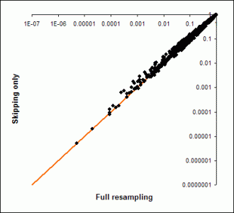
Thus, one optimization is to skip some gene sets sizes when examining large gene set sizes. Currently the exact way we do this is not settable by the user (other than to turn it off). At this writing the implementation is to start skipping some sizes when gene set sizes hit 21, and to increase the step size by 0.1 times the current gene set size. Thus the progression is 20, 23, 26… and later …69, 76, 84, 93…
The following graph shows the difference this makes for a gene-score based analysis. Note that the axes are on a log scale. This shows that for the most part, the difference in the p-value you get is minor.
2. Approximating with normal distributions.
The next approximation makes use of the central limit theorem, which states (roughly) that the distribution of means sampled from a population will tend to be normal. If you don’t know what that means, don’t worry.
To implement this, we start by using random samples, but stop when the mean and variance of the “fitted” normal distribution converge (stop changing).
As gene set sizes increase, the agreement with the normal is bound to improve. In the current implementation, the approximation kicks in for gene sets of size 10 or greater for correlation-based scoring, and 30 or greater for gene score-based analysis.
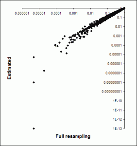
The next graph shows a comparison of the gene set p values obtained using pure resampling (100,000 samples). This shows that using this approximation tends to yield better p values (though not always). This is partly because the fit isn’t perfect, but also because the analytic distribution can yield better p values than the empirical one (which is limited by the number of samples taken; in fact here we set pvalues that came out as zero to a fixed low value so they would plot on a log scale). However, overall the results are reasonable, the ranking of gene sets will be similar, and the speed increase (especially for the correlation-based scoring) is dramatic.
Using the “Median” method for raw scores
Strictly speaking, the central limit theorem doesn’t hold for samples of the median of a population. However, for this type of data it should work reasonably well. We have not tested this extensively.

